人间正自有赖嬉戏、无邪与过剩的花朵，否则世界就太小，生趣就太枯涸。

# Untyped Lambda Calculus

Definition (The Set $\Lambda$ of Untyped λ-Terms)

Variable: If $x\in V$ , then $x\in\Lambda$ .
Application: If $M,N\in\Lambda$ , then $(M\;N)\in\Lambda$ .
Abstraction: If $x\in V$ and $M\in\Lambda$ , then $(\lambda x.M)\in\Lambda$ .

Notation(Terms)

Lowercase latin letters $x,y,z,...$ denote term variables.
Uppercase latin letters $L,M,N,...$ denote λ-terms.
Syntactical identity will be denoted with $\equiv$ .

Notation(Parentheses)

Outer most parentheses may be omitted: $(\lambda x.(M))=\lambda x.M$ .
Application is left-associative: $(M\;N)\;L\equiv M\;N\;L$ .
Abstraction is right-associative: $\lambda x.(\lambda y.M)\equiv \lambda x.\lambda y.M$ .
Application takes precedence over abstraction: $\lambda x.(M\;N)=\lambda x.M\;N$ .

Definition(The Set of Free Variables FV of a λ-Term)

Variable: $FV(x)=\{x\}$ .
Application: $FV(M\;N)=FV(M)\cup FV(N)$ .
Abstraction: $FV(\lambda x.M)=FV(M)/\{x\}$ .

Definition(α-Conversion)

Two λ-terms $M,N\in\Lambda$ are α-convertible, denoted by $M\equiv N$ , if and only if they differ only by the names of their bound variables.

Definition(Barendregt Conversion)

All bound variables in a λ-term $M\in\Lambda$ should be pairwise different and chosen such that they differ from the free variables in the term.

Definition(Substitution)

Variable: $x[x:=N]\equiv N$ . $y[x:=N]\equiv y$ if $x\neq y$ .
Application: $(P\;Q)[x:=N]\equiv (P[x:=N])\;(Q[x:=N])$ .
Abstraction: $(\lambda y.P)[x:=N]\equiv\lambda y.(P[x:=N])$ , if $y\notin FV(N)$ .

Definition(One-step β-Reduction $\rightarrow_\beta$ )

Basis: $(\lambda x.M)\;N\rightarrow_\beta M[x:=N]$ .
Compatibility: If $M\rightarrow_\beta N$ , then $M\;L\rightarrow_\beta N\;L$ , $L\;M\rightarrow_\beta L\; N$ and $\lambda x.M\rightarrow_\beta \lambda x.N$ .

Definition(Many-step β-Reduction $\rightarrow^*_\beta$ )

$M\rightarrow^*_\beta N$ if there is an $n\geq 0$ and terms $M_0,...,M_n\in\Lambda$ such that $M_0\equiv M,M_n\equiv N$ and for all $1\leq i\leq n$ :

$M_i\rightarrow_\beta M_{i+1}$

Definition(β-Conversion $=_\beta$ )

$M=_\beta N$ if there is an $n\geq 0$ and terms $M_0,...,M_n\in\Lambda$ such that $M_0\equiv M,M_n\equiv N$ and for all $1\leq i\leq n$ :

$M_i\rightarrow_\beta M_{i+1}\vee M_{i+1}\rightarrow_\beta M_i$

Definition(β-Normal Form)

$M$ is in β-normal form if $M$ does not contain any redex.
$M$ has a β-normal form if there is an $N\in\Lambda$ in β-normal form such that $M=_\beta N$ .

For example, $(\lambda x.(\lambda y.x\;y)\;z)\;v$ has a β-normal form $v\;z$ .

$\Omega=(\lambda x.x\;x)(\lambda x.x\;x)$ does not have a β-normal form.

But $(\lambda v.u)\;\Omega\rightarrow_\beta u$ or get into infinite reduction chain.

Definition(Weak Normalization, Strong Normalization)

$M$ is weakly normalizing if there is an $N\in\Lambda$ in β-normal form such that $M\rightarrow^*_\beta N$ .
$M$ is strongly normalizing if every chain of reductions starting from $M$ reaches the β-normal form.

Definition(Normalization of Systems)

A rewrite system is strongly/weakly normalizing if every term in the system is strongly/weakly normalizing. Otherwise it is not normalizing.

Theorem:

Let $M,N_1,N_2\in\Lambda$ be λ-terms with $M\rightarrow^*_\beta N_1$ and $M\rightarrow^*_\beta N_2$ .

Then there is a λ-term $N_3\in\Lambda$ such that $N_1\rightarrow^*_\beta N_3$ and $N_2\rightarrow^*_\beta N_3$ .

Definition(Natural Numbers $\mathbb{N}$ )

Zero: $0\in\mathbb{N}$ .
Successor: If $n\in\mathbb{N}$ , then $succ(n)\in\mathbb{N}$ .

Definition(Church Numerals $c_n$ )

$0=\lambda f.\lambda x.x\\ \underbrace {succ(succ(...succ(0)))}_{n-times}=\lambda f.\lambda x.\underbrace {f\;(f\;...(f\;x))}_{n-times}$

$succ\equiv \lambda m.\lambda f.\lambda x.f\;(m\;f\;x)\\ pred\equiv \lambda n.\lambda f.\lambda x.n\;(\lambda g.\lambda h.h\;(g\;f))\;(\lambda u.x)\;(\lambda u.u)\\ add\equiv \lambda m.\lambda n.\lambda f.\lambda x.m\;f\;(n\;f\;x)\\ sub\equiv \lambda m.\lambda n.(n\;pred)\;m\\ mul\equiv\lambda m.\lambda n.\lambda f.\lambda x.m\;(n\;f)\;x$

Definition(Church Booleans)

True: $T=\lambda x.\lambda y.x$ .
False: $F=\lambda x.\lambda y.y$ .

$\wedge\equiv \lambda x.\lambda y.x\;y\;F\\ \vee\equiv \lambda x.\lambda y.x\;T\;y\\ \neg\equiv \lambda x.x\;F\;T$

“if B then M else N” $\equiv B\;M\;N$ .

What’s more:

$isZero\equiv\lambda n.n\;(\lambda x.F)\;T\\ leq\equiv\lambda m.\lambda n.isZero\;(sub\;m\;n)\\ eq\equiv \lambda m.\lambda n.(leq\;m\;n)\wedge(leq\;n\;m)$

Theorem(Fixed Point Theorem):

For all $M\in\Lambda$ there exists $P\in\Lambda$ such that $M\;P=_\beta P$ .

$P\equiv (\lambda x.M\;(x\;x))\;(\lambda x.M\;(x\;x))$ . $P\rightarrow^*_\beta M\;P$ .

Definition(Combinator)

A combinator is a term without any free variables.

Definition(Fixed Point Combinator - Mathematics)

A fixed point combinator is a higher-order function that takes a function as argument and returns the fixed point of that function.

Definition(Y - Combinator)

$Y\equiv\lambda f.(\lambda x.f\;(x\;x))\;(\lambda x.f\;(x\;x))$

We have $g\;(Y\;g)=_\beta Y\;g$ . So $Y\;g$ returns a fixed point of $g$ .

Now we can compute recursive functions:

$fact'=\lambda f.\lambda x.(isZero\;x)\;1\;(mult\;x\;(f\;(pred\;x)))\\ -----------------------------\\ fact=_\beta Y\;fact'\\ =_\beta fact'\;(Y\;fact')\\ =_\beta \lambda x.(isZero\;x)\;1\;(mult\;x\;((Y\;fact')\;(pred\;x)))\\ \equiv \lambda x.(isZero\;x)\;1\;(mult\;x\;(fact\;(pred\;x)))$

Obviously it’s a weakly normalizing term.

# Simple Typed Lambda Calculus( $\lambda_\rightarrow$ )

Definition(The Set $\mathbb{T}$ of Simple Types)

Variable Type: If $\alpha\in\mathbb{V}$ , then $\alpha\in\mathbb{T}$ .
Arrow Type: If $\sigma,\tau\in\mathbb{T}$ , then $(\sigma\rightarrow\tau)\in\mathbb{T}$ .

Noticing that $V$ is the set of variables and $\mathbb{V}$ is the set of types named variable types.

Notation

$\alpha,\beta,\gamma,...$ denote type variables.
$\sigma,\tau,\rho,...$ denote arbitrary types.
Syntactical identity will be denoted with $\equiv$ .
Outermost parentheses may be omitted.
Arrow types are right-associative: $\sigma\rightarrow(\tau\rightarrow\rho)\equiv\sigma\rightarrow\tau\rightarrow\rho$ .

Definition(The Set $\Lambda^\rightarrow$ of Pre-Typed $\lambda_\rightarrow$ -Terms)

Variable: If $x\in V$ , then $x\in\Lambda^\rightarrow$ .
Application: If $M,N\in\Lambda^\rightarrow$ , then $(M\;N)\in\Lambda^\rightarrow$ .
Abstraction: If $x\in V,\sigma\in\mathbb{T}$ and $M\in\Lambda^\rightarrow$ , then $(\lambda x:\sigma.M)\in\Lambda^\rightarrow$ .

Definition

A statement is of the form $M:\sigma$ , $M$ is called the subject and $\sigma$ the type.
A declaration is a statement $x:\sigma$ .
A context $\Gamma$ is a set of declarations with different subjects.
A judgement is of the form $\Gamma\vdash M:\sigma$ .
A term $M$ is called legal if there exists $\Gamma$ and $\sigma$ such that $\Gamma\vdash M:\sigma$ .

Derivation Rules:

Type Checking: Given a context $\Gamma$ , term $M$ and type $\sigma$ , to check whether $\Gamma\vdash M:\sigma$

Well-typedness: Given a term $M$ , to find whether $?\vdash M:?$ .

Type Assignment: Given a context $\Gamma$ and a term $M$ , to find whether $\Gamma\vdash M:?$ .

Inhabitation: Given a context $\Gamma$ and a type $\sigma$ , to find whether $\Gamma\vdash ?:\sigma$ .

$\lambda_\rightarrow$ is poly-time decidable!

Definition(Domain)

The domain of a context $\Gamma=x_1:\sigma_1,..,x_n:\sigma_n$ is $dom(\Gamma)=\{x_1,...,x_n\}$ .

Lemma: If $\Gamma\vdash M:\sigma$ , then $FV(M)\subseteq dom(\Gamma)$ .

Lemma(Thinning): Let $\Gamma_1,\Gamma_2$ be contexts with $\Gamma_1\subseteq\Gamma_2$ . If $\Gamma_1\vdash M:\sigma$ , then also $\Gamma_2\vdash M:\sigma$ .

Lemma(Subterm): If $M$ is a legal term, then all subterms of $M$ are also legal terms.

Lemma(Uniqueness): If $\Gamma\vdash M:\sigma$ and $\Gamma\vdash M:\tau$ , then $\sigma\equiv\tau$ .

Definition(β-Reduction) (only for legal terms)

Basis: $(\lambda x:\sigma.M)\;N\rightarrow_\beta M[x:=N]$ .
Compatibility: If $M\rightarrow_\beta N$ , then $M\;L\rightarrow_\beta N\;L$ , $L\;M\rightarrow_\beta L\; N$ and $\lambda x:\sigma.M\rightarrow_\beta \lambda x:\sigma.N$ .

Lemma (Subject Reduction): If $\Gamma\vdash M_1:\sigma$ and $M_1\rightarrow^*_\beta M_2$ , then $\Gamma\vdash M_2:\sigma$ .

Theorem (Church-Rosser Theorem):

Let $M,N_1,N_2\in\Lambda^\rightarrow$ be simply typed λ-terms with $M\rightarrow^*_\beta N_1$ and $M\rightarrow^*_\beta N_2$ . Then there is a simply typed λ-term $N_3\in\Lambda^\rightarrow$ such that $N_1\rightarrow^*_\beta N_3$ and $N_2\rightarrow^*_\beta N_3$ .

strongly/weakly normalizing and many steps reduction are just similar to untyped ones.

Theorem (Strong Normalization Theorem):

Every legal term in $\lambda_\rightarrow$ is strongly normalizing.

Noticing that Self-application is not typable in $\lambda_\rightarrow$ .

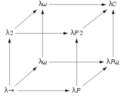
# The Extension $\lambda_2$

Definition(The Set $\mathbb{T}_2$ of $\lambda_2$ Types)

Variable Type: If $\alpha\in\mathbb{V}$ , then $\alpha\in\mathbb{T}_2$ .
Arrow Type: If $\sigma,\tau\in\mathbb{T}_2$ , then $(\sigma\rightarrow\tau)\in\mathbb{T}_2$ .
$\Pi$ -type: If $\alpha\in\mathbb{V}$ and $\sigma\in\mathbb{T}_2$ , then $(\Pi\alpha:*.\sigma)\in\mathbb{T}_2$ .

Definition(The Set $\Lambda_2$ of Pre-Typed $\lambda_2$ -Terms)

Variable: If $x\in V$ , then $x\in\Lambda_2$ .
Application: If $M,N\in\Lambda_2$ , then $(M\;N)\in\Lambda_2$ .

If $M\in\Lambda_2,\sigma\in\mathbb{T}_2$ , then $(M\;\sigma)\in\Lambda_2$ .
Abstraction: If $x\in V,\sigma\in\mathbb{T}_2$ and $M\in\Lambda_2$ , then $(\lambda x:\sigma.M)\in\Lambda_2$ .

If $\sigma\in\mathbb{V},M\in\Lambda_2$ then $(\lambda\sigma:*.M)\in\Lambda_2$ .

Definition(β-Reduction) (only for legal terms)

Basis: $(\lambda x:\sigma.M)\;N\rightarrow_\beta M[x:=N]$ .

$(\lambda\alpha:*.M)\;\sigma\rightarrow_\beta M[\alpha:=\sigma]$ .
Compatibility: If $M\rightarrow_\beta N$ , then $M\;L\rightarrow_\beta N\;L$ , $L\;M\rightarrow_\beta L\; N$ and $\lambda x:\sigma.M\rightarrow_\beta \lambda x:\sigma.N$ .

Definition

A statement is of the form $M:\sigma$ , $M$ is called the subject and $\sigma$ the type.
A term declaration is a statement $x:\sigma$ .
A type declaration is of the form $\sigma:*$ .
A context $\Gamma$ is a set of declarations with different subjects.
A judgement is of the form $\Gamma\vdash M:\sigma$ .
A term $M$ is called legal if there exists $\Gamma$ and $\sigma$ such that $\Gamma\vdash M:\sigma$ .

Notice! In a valid $\lambda_2$ -context every type variable $\sigma$ is declared $(\sigma:*)$ before it is used $(M:\sigma)$ .

Derivation Rules:

$\Gamma\vdash x:\sigma\quad if\;x:\sigma\in\Gamma\quad(var)\\ \frac{\Gamma\vdash M:\sigma\rightarrow\tau\quad\Gamma\vdash N:\sigma}{\Gamma\vdash M\;N:\tau}\quad(appl)\\ \frac{\Gamma,x:\sigma\vdash M:\tau}{\Gamma\vdash\lambda x:\sigma.M:\sigma\rightarrow\tau}\quad(abst)\\ \Gamma\vdash B:*\quad if\; B\in\mathbb{T}_2\;and\;all\;free\;type\;variables\;in\\ B\;are\;declared\;in\;\Gamma\quad(form)\\ \frac{\Gamma,\alpha:*\vdash M:A}{\Gamma\vdash(\lambda\alpha:*.M):(\Pi\alpha:*.A)}\quad(abst_2)\\ \frac{\Gamma\vdash M:(\Pi\alpha:*.A)\quad\Gamma\vdash B:*}{\Gamma\vdash M\;B:A[\alpha:=B]}\quad(appl_2)$

Definition(Type of Church Numerals)

$\mathcal{C}\equiv\Pi\alpha:*.(\alpha\rightarrow\alpha)\rightarrow\alpha\rightarrow\alpha$

Definition(Pair of Church Numerals)

$\langle M,N\rangle\equiv\lambda z:\mathcal{C}\rightarrow\mathcal{C}\rightarrow\mathcal{C}.z\;M\;N:(\mathcal{C}\rightarrow\mathcal{C}\rightarrow\mathcal{C})\rightarrow\mathcal{C}\\ pair\equiv(\mathcal{C}\rightarrow\mathcal{C}\rightarrow\mathcal{C})\rightarrow\mathcal{C}\\ fst\equiv\lambda p:pair.p\;(\lambda x:\mathcal{C}.\lambda y:\mathcal{C}.x)\\ snd\equiv\lambda p:pair.p\;(\lambda x:\mathcal{C}.\lambda y:\mathcal{C}.y)$

Now we can reconsider the factorial function:

$next\;\langle n,fact\;n\rangle\rightarrow\langle n+1,fact\;n+1\rangle$

where

$next=\lambda p:pair.\langle succ\;(fst\;p),mult\;(succ\;(fst\;p))\;(snd\;p)\rangle\\ next:pair\rightarrow pair$

So $\langle n,fact(n)\rangle=_\beta next^n\;\langle 0,1\rangle$ . It comes back to the form:

$\lambda\alpha:*.\lambda f:\alpha\rightarrow\alpha.\lambda x:\alpha.f^n\;x:\Pi\alpha:*.(\alpha\rightarrow\alpha)\rightarrow\alpha\rightarrow\alpha$

What’s interesting, the type is church numerical type! so

$c_n\;pair\;next\;\langle 0,1\rangle=_\beta\langle c_n,fact\;c_n\rangle$

where $c_n$ is church numerical. So

$fact\equiv \lambda n:\mathcal{C}.snd\;(n\;pair\;next\;\langle 0,1\rangle):\mathcal{C}\rightarrow\mathcal{C}$

Church numbers can represent loop somehow.

# The Extension $\lambda\underline{\omega}$ (Lambda Weak Omega)

Definition(The Set $\mathbb{K}$ of All Kinds)

$\mathbb{K}=*\;|\;(\mathbb{K}\rightarrow\mathbb{K})$ .

$term:type:kind:sort:\Box$ .

Noticing that $\lambda\underline{\omega}$ doesn’t support polymorphism, as a matter of fact, such type $\Pi\alpha:*.\alpha$ is illegal.

However, if we want to combine polymorphism into lambda weak omega, we need to noticing the difference between $*\rightarrow *$ and $\Pi\alpha:*,\alpha\rightarrow\alpha$ :

we can write:

$(\lambda\alpha:*.\lambda x:\alpha.x):(\Pi\alpha:*.\alpha\rightarrow\alpha):*$

since $\Pi\alpha:*.\alpha\rightarrow \alpha$ is a specific type, so its kind is $*$ .

while $\lambda\alpha:*.\alpha\rightarrow\alpha:*\rightarrow *$ , it’s considered as the type constructor.

$(\lambda \alpha:*.\lambda x:\alpha.x):(\lambda \alpha:*.\alpha\rightarrow\alpha)$ is wrong!

$(\lambda \alpha:*.\lambda x:\alpha.x):*\rightarrow *$ is wrong!

Derivation Rules:

$\empty\vdash *:\Box\quad(sort)\\ \frac{\Gamma\vdash A:s}{\Gamma,x:A\vdash x:A}if\;x\notin\Gamma\quad(var)\\ \frac{\Gamma\vdash A:B\quad\Gamma\vdash C:s}{\Gamma,x:C\vdash A:B}if\;x\notin\Gamma\quad (weak)\\ \frac{\Gamma\vdash A:s\quad\Gamma\vdash B:s}{\Gamma\vdash A\rightarrow B:s}\quad(form)\\ \frac{\Gamma\vdash M:A\rightarrow B\quad \Gamma\vdash N:A}{\Gamma\vdash M\;N:B}\quad(appl)\\ \frac{\Gamma,x:A\vdash M:B\quad\Gamma\vdash A\rightarrow B:s}{\Gamma\vdash \lambda x:A.M:A\rightarrow B}\quad (abst)\\ \frac{\Gamma\vdash A:B\quad \Gamma\vdash B':s}{\Gamma\vdash A:B'}if\;B=_\beta B'\quad(conv)$

L1	L2	L3	L4
$\lambda x:\alpha.x$ (terms)	$\alpha\rightarrow\alpha$ (type)	$*$ (kind)	$\Box$ (sort)
	$\lambda \alpha:*.\alpha$ (type constructor)	$\rightarrow $ (kind)	$\Box$ (sort)

The derivation rules seem strange in that the only axiom is $*:\Box$ , which is the relation between L3 and L4.

And we can derive:

$\frac{\empty\vdash *:\Box}{\sigma:*\vdash\sigma:*}\quad(var)$

it’s the relation between L2 and L3.

And we can derive:

$\frac{\sigma:*\vdash\sigma:*}{\sigma:*,x:\sigma\vdash x:\sigma}\quad (var)$

it’s the relation between L1 and L2.

So we can discover that the derivation rule var can be applied between any two adjacent layers.

Similarly, In weak derivation rule, $x$ can be types or terms.

In form rules, $A$ can be types or kinds.

In appl rules, $M$ can be terms or type constructors.

In abst rules, $A$ can be types or kinds.

$\Gamma \vdash\sigma:*$ means $\sigma$ is a well-formed type. $\Gamma\vdash\lambda \alpha:*.\alpha:*\rightarrow *$ means $\lambda \alpha:*.\alpha$ is a well-formed type constructor. $\Gamma\vdash *\rightarrow *:\Box$ means $*\rightarrow *$ is a well-formed kind.

# The Extension $\lambda_P$ (Lambda P)

Derivation Rules:

$\empty\vdash *:\Box\quad(sort)\\ \frac{\Gamma\vdash A:s}{\Gamma,x:A\vdash x:A}if\;x\notin\Gamma\quad(var)\\ \frac{\Gamma\vdash A:B\quad\Gamma\vdash C:s}{\Gamma,x:C\vdash A:B}if\;x\notin\Gamma\quad (weak)\\ \frac{\Gamma\vdash A:*\quad\Gamma,x:A\vdash B:s}{\Gamma\vdash\Pi x:A.B:s}\quad(form)\\ \frac{\Gamma\vdash M:\Pi x:A.B\quad \Gamma\vdash N:A}{\Gamma\vdash M\;N:B[x:=N]}\quad(appl)\\ \frac{\Gamma,x:A\vdash M:B\quad\Gamma\vdash A\rightarrow B:s}{\Gamma\vdash \lambda x:A.M:A\rightarrow B}\quad (abst)\\ \frac{\Gamma\vdash A:B\quad \Gamma\vdash B':s}{\Gamma\vdash A:B'}if\;B=_\beta B'\quad(conv)$

# Propositions as Types

PAT: Propositions As Types and Proofs As Terms

$M:\sigma$ , $M$ corresponds to a proof and $\sigma$ corresponds to a proposition.

$\sigma$ is inhabited $\Leftrightarrow$ $P$ is proved.

# Untyped Lambda Calculus

# Simple Typed Lambda Calculus(λ→\lambda_\rightarrowλ→​)

# The Extension λ2\lambda_2λ2​

# The Extension λω‾\lambda\underline{\omega}λω​ (Lambda Weak Omega)

# The Extension λP\lambda_PλP​ (Lambda P)

# Propositions as Types

睡美人

Category theory

# Simple Typed Lambda Calculus( $\lambda_\rightarrow$ )

# The Extension $\lambda_2$

# The Extension $\lambda\underline{\omega}$ (Lambda Weak Omega)

# The Extension $\lambda_P$ (Lambda P)